MLP-Mixer re-invented for auto-encoding ←
Recently read this paper "MLP-Mixer: An all-MLP Architecture for Vision" 2105.01601, which i found quite inspiring but also left me with some regret of not having come up with it myself.
Anyways, after some weeks, i set out to program a network based on the ideas but without looking at the paper for reference. At least before i have a performing implementation. Of course, because i like auto-encoders so much, i used it for auto-encoding.
Setup is as follows:
First split the input image into equal sized patches. I'm using pytorch's unfold method for this.
For the MNIST digits dataset this yield 4x4 7x7 patches for each 28x28 image.
Then they are flattened to 16 1-D vectors of size 49. Those vectors are moved to the batch-dimension (the first one) of the vector that the linear layers ought to process. For example, when passing in a batch-size of 64 (64 images at once):
input:                      (64, 1, 28, 28)
patches:                    (64, 4, 4, 1, 7, 7)
flatten:                    (64, 16, 49)
move to batch dimension:    (1024, 49)
Now these 1024 49-D vectors can be processed by a stack of linear layers (MLP). Each vector is processed by the same layer and since it's only one little patch, the linear layer can be very small. However, there is no information shared between those patches. Each patch is processed individually. To apply the "mixing" strategy, i first tried a 1-D convolutional layer
input:                      (1024, 49)
reverse batch-flattening:   (64, 16, 49)
apply Conv1d(16, 16, 1):    (64, 16, 49)
move to batch dimension:    (1024, 49)
process further with MLP:   (1024, 49)
The convolution is applied channel-wise and is able to mix information from the different patches.
Note that the 49 is the depth of each layer and does not have to stay like this. Each linear
layer can make it larger or smaller. In the following experiment, i resized the 49 to 64 in the
first layer and kept it like this until the final linear layer, which resizes it to 16 which yields
a compression ratio of 49 (28x28 -> 49) for the auto-encoder.
Also, whenever a layer has the same input and output dimension, a residual connection is added (after the activation function).
The whole auto-encoder is built symmetrically, so the decoder stack is the reverse of the encoder stack. Here is one example in pytorch speak:
MixerMLP(
  (patchify): Patchify(patch_size=7)
  (encoder): ModuleList(
    (0): MLPLayer(
      residual=False
      (module): Linear(in_features=49, out_features=64, bias=True)
      (act): GELU(approximate='none')
    )
    (1): MLPLayer(
      residual=True
      (module): Linear(in_features=64, out_features=64, bias=True)
      (act): GELU(approximate='none')
    )
    (2): MLPMixerLayer(
      residual=True
      (module): Conv1d(16, 16, kernel_size=(1,), stride=(1,))
    )
    (3): MLPLayer(
      residual=True
      (module): Linear(in_features=64, out_features=64, bias=True)
      (act): GELU(approximate='none')
    )
    (4): MLPMixerLayer(
      residual=True
      (module): Conv1d(16, 16, kernel_size=(1,), stride=(1,))
    )
    (5): MLPLayer(
      residual=False
      (module): Linear(in_features=64, out_features=16, bias=True)
      (act): GELU(approximate='none')
    )
    (6): MLPMixerLayer(
      residual=True
      (module): Conv1d(16, 16, kernel_size=(1,), stride=(1,))
    )
    (7): MLPLayer(
      residual=False
      (module): Linear(in_features=256, out_features=16, bias=True)
    )
  )
  (decoder): ModuleList(
    (0): MLPLayer(
      residual=False
      (module): Linear(in_features=16, out_features=256, bias=True)
    )
    (1): MLPMixerLayer(
      residual=True
      (module): Conv1d(16, 16, kernel_size=(1,), stride=(1,))
      (act): GELU(approximate='none')
    )
    (2): MLPLayer(
      residual=False
      (module): Linear(in_features=16, out_features=64, bias=True)
      (act): GELU(approximate='none')
    )
    (3): MLPMixerLayer(
      residual=True
      (module): Conv1d(16, 16, kernel_size=(1,), stride=(1,))
      (act): GELU(approximate='none')
    )
    (4): MLPLayer(
      residual=True
      (module): Linear(in_features=64, out_features=64, bias=True)
      (act): GELU(approximate='none')
    )
    (5): MLPMixerLayer(
      residual=True
      (module): Conv1d(16, 16, kernel_size=(1,), stride=(1,))
      (act): GELU(approximate='none')
    )
    (6): MLPLayer(
      residual=True
      (module): Linear(in_features=64, out_features=64, bias=True)
      (act): GELU(approximate='none')
    )
    (7): MLPLayer(
      residual=False
      (module): Linear(in_features=64, out_features=49, bias=True)
    )
  )
  (unpatchify): Unpatchify(patch_size=7)
)
Note that, in the encoder, layer 5 compresses each patch from 64 to 16 dimensions, then there is another mixing layer, and layer 7 processes all 16 patches at once and outputs a final 16-dim vector (256 -> 16).
As with other MLPs, this auto-encoder is input-size-dependent. The network is constructed for a fixed image size and can not be used for other sizes.
In the following table bs = batch size, lr = learnrate, ds is the dataset, ps is the patch size,
mix means at which layer a mixing-layer is added (1-indexed). Optimizer is AdamW and loss function
is mean-squared error. Scheduler is cosine-annealing with warmup.
Experiment file: experiments/ae/mixer/mixer02.yml @ 18e32d81
| bs | lr | ds | ps | ch | mix | act | validation loss (1,000,000 steps) |
model params | train time (minutes) | throughput |
|---|---|---|---|---|---|---|---|---|---|---|
| 64 | 0.003 | mnist | 7 | 64,64,64,16 | gelu | 0.011366 | 33,617 | 1.03 | 16,126/s | |
| 64 | 0.003 | mnist | 7 | 64,64,64,16 | 4 | gelu | 0.011248 | 34,161 | 1.25 | 13,335/s |
| 64 | 0.003 | mnist | 7 | 64,64,64,16 | 3 | gelu | 0.010779 | 34,161 | 1.21 | 13,779/s |
| 64 | 0.003 | mnist | 7 | 64,64,64,16 | 2 | gelu | 0.010677 | 34,161 | 1.2 | 13,865/s |
| 64 | 0.003 | mnist | 7 | 64,64,64,16 | 1 | gelu | 0.010659 | 34,161 | 1.21 | 13,748/s |
| 64 | 0.003 | mnist | 7 | 64,64,64,16 | 1,2 | gelu | 0.010418 | 34,705 | 1.29 | 12,883/s |
| 64 | 0.003 | mnist | 7 | 64,64,64,16 | 1,2,3 | gelu | 0.010398 | 35,249 | 1.46 | 11,384/s |
| 64 | 0.003 | mnist | 7 | 64,64,64,16 | 1,2,3,4 | gelu | 0.010208 | 35,793 | 1.61 | 10,323/s |
Validation loss performance is not actually super good and the mixing only helps a little. But it's not so bad either for such a small network.
Linear layer as mixer ←
So let's try a linear layer for mixing between patches.
input:                      (1024, 49)
reverse batch-flattening:   (64, 16, 49)
flatten 2nd dimension:      (64, 784)
apply Linear(784, 784):     (64, 784)
unflatten 2nd dimension:    (64, 16, 49)
and move to batch dim:      (1024, 49)
process further with MLP:   (1024, 49)
Obviously, the linear mixing layer increases the network size considerably. The benefit is, that each pixel in each patch can be compared/processed against each other.
I guess, this is kind of what the MLP-Mixer paper suggests, only i can not confidentially read their jax code to confirm.
| bs | lr | ds | ps | ch | mix | act | validation loss (1,000,000 steps) |
model params | train time (minutes) | throughput |
|---|---|---|---|---|---|---|---|---|---|---|
| 64 | 0.003 | mnist | 7 | 64,64,64,16 | 4 | gelu | 0.0105164 | 165,201 | 1.16 | 14,418/s |
| 64 | 0.003 | mnist | 7 | 64,64,64,16 | 1 | gelu | 0.0078778 | 2,132,817 | 1.17 | 14,292/s |
| 64 | 0.003 | mnist | 7 | 64,64,64,16 | 2 | gelu | 0.0072450 | 2,132,817 | 1.16 | 14,345/s |
| 64 | 0.003 | mnist | 7 | 64,64,64,16 | 3 | gelu | 0.0071680 | 2,132,817 | 1.21 | 13,793/s |
| 64 | 0.003 | mnist | 7 | 64,64,64,16 | 3,4 | gelu | 0.0069653 | 2,264,401 | 1.41 | 11,778/s |
| 64 | 0.003 | mnist | 7 | 64,64,64,16 | 1,2 | gelu | 0.0068538 | 4,232,017 | 1.58 | 10,559/s |
| 64 | 0.003 | mnist | 7 | 64,64,64,16 | 1,2,3,4 | gelu | 0.0066289 | 6,462,801 | 2.06 | 8,083/s |
| 64 | 0.003 | mnist | 7 | 64,64,64,16 | 1,2,3 | gelu | 0.0065175 | 6,331,217 | 1.87 | 8,894/s |
| 64 | 0.003 | mnist | 7 | 64,64,64,16 | 2,3,4 | gelu | 0.0065056 | 4,363,601 | 1.62 | 10,303/s |
Here's a plot of the loss curves for both mixing methods:
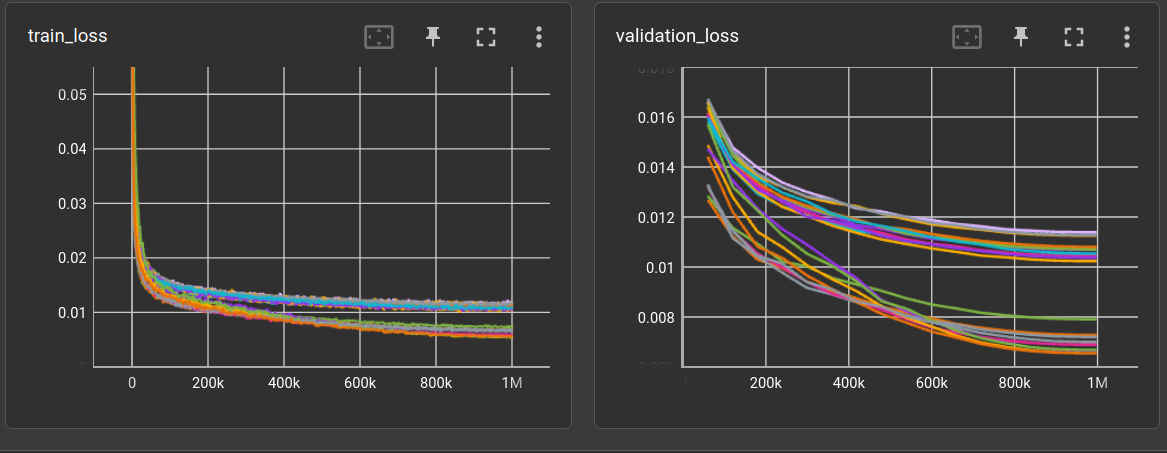
Performance is much better but the number of model parameters is much larger as well.
Comparison with baseline CNN ←
How well does it perform against a baseline CNN with a final linear layer?
EncoderDecoder(
  (encoder): EncoderConv2d(
    (convolution): Conv2dBlock(
      (layers): Sequential(
        (0): Conv2d(1, 24, kernel_size=(5, 5), stride=(1, 1))
        (1): ReLU()
        (2): Conv2d(24, 32, kernel_size=(5, 5), stride=(1, 1))
        (3): ReLU()
        (4): Conv2d(32, 48, kernel_size=(5, 5), stride=(1, 1))
        (5): ReLU()
      )
    )
    (linear): Linear(in_features=12288, out_features=16, bias=True)
  )
  (decoder): Sequential(
    (0): Linear(in_features=16, out_features=12288, bias=True)
    (1): Reshape(shape=(48, 16, 16))
    (2): Conv2dBlock(
      (layers): Sequential(
        (0): ConvTranspose2d(48, 32, kernel_size=(5, 5), stride=(1, 1))
        (1): ReLU()
        (2): ConvTranspose2d(32, 24, kernel_size=(5, 5), stride=(1, 1))
        (3): ReLU()
        (4): ConvTranspose2d(24, 1, kernel_size=(5, 5), stride=(1, 1))
      )
    )
  )
)
ks is kernel size
| ch | ks | validation loss (1,000,000 steps) |
model params | train time (minutes) | throughput |
|---|---|---|---|---|---|
| 24,32,48 | 9 | 0.00780634 | 402,657 | 1.87 | 8,914/s |
| 24,32,48 | 7 | 0.00710207 | 386,721 | 1.44 | 11,557/s |
| 24,32,48 | 3 | 0.00718373 | 808,737 | 2.11 | 7,908/s |
| 24,32,48 | 5 | 0.00655708 | 522,081 | 1.93 | 8,643/s |
Seems to be equally good at first glance. However, training both networks a bit longer reveals that the CNN is able to squeeze out some more performance:
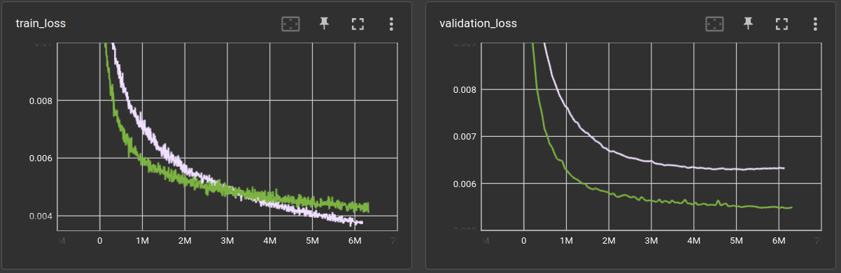
After 6 million steps (or 100 epochs), the best performing Mixer-MLP from above archives a validation loss of 0.0063 vs. 0.0055 for the CNN model.
The Mixer-MLP is 4 times larger than the CNN model (because of the 3 linear mixing stages) and we can see from the loss curves that it actually overfitted the training set. It's validation performance starts to get worse after 5 million steps.
However, since it seems to behave quite differently to the baseline CNN, it's certainly a nice new tool to try things on.
It would be interesting to see if the mixing stages implemented with a convolution, can--somehow--reach the performance of the fully connected linear mixers. That would make it very small and powerful.
Tweaking the convolutional mixing stage ←
First of all, we can use a larger kernel size than 1. That would allow the mixing stage to correlate nearby pixels of individual patches. Since it's a 1-D convolution that would still only correlate pixels left and right and not the ones above and below.
Secondly we might use 2 convolutions. One that mixes the patches and one that mixes the pixels. Following the example above, that would look like:
input:                      (1024, 49)
reverse batch-flattening:   (64, 16, 49)
apply Conv1d(16, 16):       (64, 16, 49)
transpose vector:           (64, 49, 16)
apply Conv1d(49, 49):       (64, 49, 16)
transpose vector:           (64, 16, 49)
move to batch dimension:    (1024, 49)
process further with MLP:   (1024, 49)
And thirdly, we could actually do a 2-dimensional convolutional mixing:
input:                      (1024, 49)
reverse batch-flattening:   (64, 16, 49)
restore 2-D patches:        (64, 16, 7, 7)
apply Conv2d(16, 16):       (64, 16, 7, 7)
flatten the patches:        (64, 16, 49)
move to batch dimension:    (1024, 49)
process further with MLP:   (1024, 49)
However, since the final dimension is not actually fixed at 49 (7x7) but can be anything, it does not really represent the 2-dimensional patch content but rather just the computational breadth of the MLP stack at each layer. We might still treat it as spatial, and let the network figure out some good way to use it.
Fourthly, if that is even a word, we can combine the two-consecutive-convolution method with the 2-D convolution which puts another constraint on the number of patches resulting from the input image: It also has to be a square number. It gets a bit complicated then:
input:                      (1024, 49)
reverse batch-flattening:   (64, 16, 49)
restore 2-D patches:        (64, 16, 7, 7)
apply Conv2d(16, 16, 1):    (64, 16, 7, 7)
flatten patches:            (64, 16, 49)
transpose dimensions:       (64, 49, 16)
make "breadth" 2-dim:       (64, 49, 4, 4)
apply Conv2d(49, 49, 1):    (64, 49, 4, 4)
flatten "breadth" dim:      (64, 49, 16)
transpose dimensions:       (64, 16, 49)
move to batch dimension:    (1024, 49)
process further with MLP:   (1024, 49)
Okay, lets test all the methods with different kernel sizes from 1 to 13. The padding of the
convolution is adjusted ((ks - 1) // 2) so the convolutions always produce the same output size.
In below table mixtype is either:
cnn: The 1-D convolution used in the beginningcnnf: two 1-D convolutions with patch/channel flipping in betweencnn2d: 2-D convolutioncnnf2d: two 2-D convolutions with patch/channel flipping in between
| bs | lr | ds | ps | ch | mix | mixtype | ks | act | validation loss (1,000,000 steps) |
model params | train time (minutes) | throughput |
|---|---|---|---|---|---|---|---|---|---|---|---|---|
| 64 | 0.003 | mnist | 7 | 64,64,64,16 | 2,3,4 | cnn | 1 | gelu | 0.0105176 | 35,249 | 1.53 | 10,866/s |
| 64 | 0.003 | mnist | 7 | 64,64,64,16 | 2,3,4 | cnn2d | 1 | gelu | 0.0103852 | 35,249 | 1.45 | 11,517/s |
| 64 | 0.003 | mnist | 7 | 64,64,64,16 | 2,3,4 | cnn | 3 | gelu | 0.0101478 | 38,321 | 1.46 | 11,447/s |
| 64 | 0.003 | mnist | 7 | 64,64,64,16 | 2,3,4 | cnn | 5 | gelu | 0.0097217 | 41,393 | 1.50 | 11,076/s |
| 64 | 0.003 | mnist | 7 | 64,64,64,16 | 2,3,4 | cnn2df | 1 | gelu | 0.0096381 | 52,433 | 2.09 | 7,989/s |
| 64 | 0.003 | mnist | 7 | 64,64,64,16 | 2,3,4 | cnnf | 1 | gelu | 0.0095420 | 52,433 | 1.90 | 8,772/s |
| 64 | 0.003 | mnist | 7 | 64,64,64,16 | 2,3,4 | cnn | 7 | gelu | 0.0095143 | 44,465 | 1.42 | 11,726/s |
| 64 | 0.003 | mnist | 7 | 64,64,64,16 | 2,3,4 | cnn | 9 | gelu | 0.0094267 | 47,537 | 1.45 | 11,489/s |
| 64 | 0.003 | mnist | 7 | 64,64,64,16 | 2,3,4 | cnn2d | 3 | gelu | 0.0093458 | 47,537 | 1.65 | 10,115/s |
| 64 | 0.003 | mnist | 7 | 64,64,64,16 | 2,3,4 | cnn | 11 | gelu | 0.0092456 | 50,609 | 1.47 | 11,327/s |
| 64 | 0.003 | mnist | 7 | 64,64,64,16 | 2,3,4 | cnn | 13 | gelu | 0.0092080 | 53,681 | 1.50 | 11,107/s |
| 64 | 0.003 | mnist | 7 | 64,64,64,16 | 2,3,4 | cnn2d | 5 | gelu | 0.0086525 | 72,113 | 1.79 | 9,292/s |
| 64 | 0.003 | mnist | 7 | 64,64,64,16 | 2,3,4 | cnn2d | 7 | gelu | 0.0083488 | 108,977 | 1.87 | 8,911/s |
| 64 | 0.003 | mnist | 7 | 64,64,64,16 | 2,3,4 | cnn2d | 9 | gelu | 0.0080035 | 158,129 | 2.05 | 8,120/s |
| 64 | 0.003 | mnist | 7 | 64,64,64,16 | 2,3,4 | cnnf | 3 | gelu | 0.0079969 | 89,297 | 1.98 | 8,404/s |
| 64 | 0.003 | mnist | 7 | 64,64,64,16 | 2,3,4 | cnn2d | 13 | gelu | 0.0077707 | 293,297 | 2.02 | 8,240/s |
| 64 | 0.003 | mnist | 7 | 64,64,64,16 | 2,3,4 | cnn2d | 11 | gelu | 0.0077622 | 219,569 | 1.88 | 8,865/s |
| 64 | 0.003 | mnist | 7 | 64,64,64,16 | 2,3,4 | cnnf | 5 | gelu | 0.0075978 | 126,161 | 2.31 | 7,211/s |
| 64 | 0.003 | mnist | 7 | 64,64,64,16 | 2,3,4 | cnnf | 7 | gelu | 0.0073687 | 163,025 | 2.47 | 6,740/s |
| 64 | 0.003 | mnist | 7 | 64,64,64,16 | 2,3,4 | cnn2df | 3 | gelu | 0.0071530 | 199,889 | 2.12 | 7,855/s |
| 64 | 0.003 | mnist | 7 | 64,64,64,16 | 2,3,4 | cnnf | 9 | gelu | 0.0071354 | 199,889 | 2.62 | 6,351/s |
| 64 | 0.003 | mnist | 7 | 64,64,64,16 | 2,3,4 | cnnf | 13 | gelu | 0.0070266 | 273,617 | 2.87 | 5,815/s |
| 64 | 0.003 | mnist | 7 | 64,64,64,16 | 2,3,4 | cnnf | 11 | gelu | 0.0070069 | 236,753 | 2.52 | 6,625/s |
| 64 | 0.003 | mnist | 7 | 64,64,64,16 | 2,3,4 | cnn2df | 5 | gelu | 0.0068095 | 494,801 | 2.35 | 7,086/s |
| 64 | 0.003 | mnist | 7 | 64,64,64,16 | 2,3,4 | cnn2df | 13 | gelu | 0.0067350 | 3,149,009 | 7.85 | 2,123/s |
| 64 | 0.003 | mnist | 7 | 64,64,64,16 | 2,3,4 | cnn2df | 11 | gelu | 0.0066938 | 2,264,273 | 6.05 | 2,755/s |
| 64 | 0.003 | mnist | 7 | 64,64,64,16 | 2,3,4 | cnn2df | 9 | gelu | 0.0066766 | 1,526,993 | 4.45 | 3,745/s |
| 64 | 0.003 | mnist | 7 | 64,64,64,16 | 2,3,4 | cnn2df | 7 | gelu | 0.0066100 | 937,169 | 2.43 | 6,872/s |
Okay, first of all, just increasing the kernel size is not so helpful. As stated above, it
only connects pixels left and right but not the once above and below. The cnn mixer archives
a validation loss between 0.01 and 0.0092 for kernel sizes 1 to 13.
The second option: Two convolutions for mixing (cnnf) work pretty good in comparison. The losses
range between 0.0095 and 0.007 for the different kernel sizes.
Third option (cnn2d): The spatial 2-D convolutions work okayish. They range between
0.01 (similar to first option with kernel size 1) and 0.0078.
It should be noted, that the huge kernel sizes do not make much sense in this example.
The spatial patches are either 7x7 or 4x4. It would make a difference for
larger input sizes, though.
Forth option (cnn2df): Two spatial convolutions work best in this example. The losses range
between 0.0096 (similar to cnnf) and 0.0066. Almost reaching the performance of the
network with fully connected linear mixers, while being much smaller in number of parameters
(at least the kernel size 7 one).
So, lets look what happens when processing something larger than the MNIST digit set.
Increasing resolution ←
In ML-papers, when larger images are required, it's almost always the ImageNet dataset that is used. Well, i sent them a request but got never got an answer. If it's just about auto-encoding, one can just crawl the web for a hundredthousand random images but this diminishes reproducibility.
So i chose the Unsplash Lite dataset, although it has some minor issues at the moment.
These are about 25,000 images, which i scaled down to 160 pixels for the longest edge, but at least 96 pixels for the smallest edge and randomly cropped 96x96 patches for training. The first 100 images are used for validation and they are center-cropped to 96x96.
To keep the auto-encoder compression ratio of 49 for comparison, the latent code has a size
of 564 (3*96*96 / 564 = 49.0213).
First, i tried different patch sizes with the cnn and cnnf mixers.
| bs | lr | ds | ps | ch | mix | mixt | ks | act | validation loss (1,000,000 steps) |
model params | train time (minutes) | throughput |
|---|---|---|---|---|---|---|---|---|---|---|---|---|
| 64 | 0.0003 | unsplash | 32 | 64,64,64,564 | 2,3,4 | cnn | 3 | gelu | 0.0073214 | 6,218,692 | 10.03 | 1,660/s |
| 64 | 0.0003 | unsplash | 32 | 64,64,64,564 | 2,3,4 | cnnf | 3 | gelu | 0.0057957 | 8,177,804 | 10.27 | 1,622/s |
| 64 | 0.0003 | unsplash | 16 | 64,64,64,564 | 2,3,4 | cnn | 3 | gelu | 0.0034742 | 23,135,920 | 11.07 | 1,505/s |
| 64 | 0.0003 | unsplash | 16 | 64,64,64,564 | 2,3,4 | cnnf | 3 | gelu | 0.0033309 | 25,095,032 | 11.63 | 1,432/s |
| 64 | 0.0003 | unsplash | 8 | 64,64,64,564 | 2,3,4 | cnn | 3 | gelu | 0.0032881 | 92,181,832 | 19.27 | 864/s |
| 64 | 0.0003 | unsplash | 8 | 64,64,64,564 | 2,3,4 | cnnf | 3 | gelu | 0.0031301 | 94,140,944 | 32.87 | 507/s |
Whoa, what happened here? First of all, the number of parameters is huge in comparison, and then the validation loss beats every previous model run on the MNIST digits dataset. Let's look closer at both phenomena.
The increased parameter count can be blamed to mostly a single layer. Look at the encoder of the patch-size-8 model:
(patchify): Patchify(patch_size=8)
(encoder): ModuleList(
    (0): MLPLayer(
      residual=False
      (module): Linear(in_features=192, out_features=64, bias=True)
      (act): GELU(approximate='none')
    )
    (1): MLPLayer(
      residual=True
      (module): Linear(in_features=64, out_features=64, bias=True)
      (act): GELU(approximate='none')
    )
    (2): MLPMixerLayer(
      residual=True
      (module): Conv1d(144, 144, kernel_size=(3,), stride=(1,), padding=(1,))
      (act): GELU(approximate='none')
    )
    (3): MLPLayer(
      residual=True
      (module): Linear(in_features=64, out_features=64, bias=True)
      (act): GELU(approximate='none')
    )
    (4): MLPMixerLayer(
      residual=True
      (module): Conv1d(144, 144, kernel_size=(3,), stride=(1,), padding=(1,))
      (act): GELU(approximate='none')
    )
    (5): MLPLayer(
      residual=False
      (module): Linear(in_features=64, out_features=564, bias=True)
      (act): GELU(approximate='none')
    )
    (6): MLPMixerLayer(
      residual=True
      (module): Conv1d(144, 144, kernel_size=(3,), stride=(1,), padding=(1,))
      (act): GELU(approximate='none')
    )
    (7): MLPLayer(
      residual=False
      (module): Linear(in_features=81216, out_features=564, bias=True)
    )
)
The 96x96 images are sliced into 144 8x8 patches.
The convolutions require 144 * 144 * 3 * 3 = 186,624 parameters each (+ the bias) so their
size is acceptable.
The fifth layer expands to hidden dimension of 564 and the final mixdown-to-latent-code
layer (lets call it head) gets a 144 * 564 vector as input and mixes it down to 564:
81216 * 564 = 45,805,824! The decoder has the same thing in reverse. That's completely
exagerated for the head of a otherwise tiny network.
Quite obviously, there is no need to expand the hidden dimensions to 564 before the head. That was just how i wrote the code without thinking too much when the networks were small. That needs to be fixed.
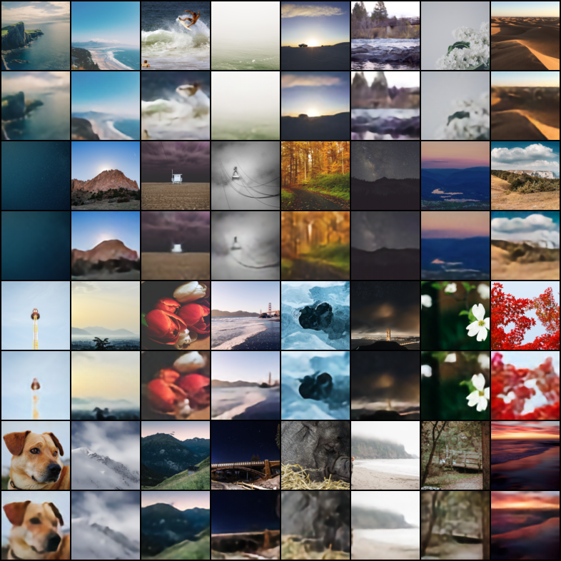
So what about the validation loss of around 0.003? Turns out that photos generally yield a lower reconstruction error compared to the high-contrast black and white MNIST digits. It does not look too great, though:

(original on top, reconstruction below)
To fix the problem with the large final layer, there is now one additonal channel number in the model configuration, which defines the breath of the final layer before the head. To keep the networks small, i used 32 (or 36 to make it square for the 2-D convolutions). Here a are a few other setups:
| bs | lr | ds | ps | ch | mix | mixt | ks | act | validation loss (1,000,000 steps) |
model params | train time (minutes) | throughput |
|---|---|---|---|---|---|---|---|---|---|---|---|---|
| 64 | 0.0003 | unsplash | 8 | 144,144,144,36,564 | 2,3,4 | cnn2df | 7 | gelu | 0.0544467 | 16,292,160 | 37.2 | 448/s |
| 64 | 0.0001 | unsplash | 8 | 144x9...,36,564 | 2,4,6,8 | cnn2df | 7 | gelu | 0.0036219 | 22,512,888 | 60.97 | 273/s |
| 64 | 0.0003 | unsplash | 8 | 64,64,64,32,564 | 2,3,4 | cnnf | 3 | gelu | 0.0033642 | 5,678,388 | 10.78 | 1,546/s |
| 64 | 0.0003 | unsplash | 8 | 64,64,64,32,564 | 2,3,4 | cnnf | 13 | gelu | 0.0033175 | 7,106,868 | 12.61 | 1,322/s |
| 64 | 0.0003 | unsplash | 8 | 64,64,64,36,564 | 2,3,4 | cnn2df | 7 | gelu | 0.0032664 | 12,926,880 | 23.34 | 713/s |
The networks are still pretty big, which feels unjustified when trusting my gut feelings. There
is also no increase in performance using the 2-D convolutions or making the network deeper
(the 144x9... means an mlp with 9 layers of 144 channels each). It actually starts to feel
like a waste of energy, literally.
Just to see what else is possible i compare against some recent "baseline" CNN-only
model that uses no MLP layers but instead decreases the spatial resolution via torch's
PixelUnshuffle method.
This move parts of the spatial pixels into the channels dimension,
which can be gradually decreased to match a certain compression ratio. In this case, the
network transforms the 3x96x96 to 1x24x24, which corresponds to a ratio of 48.
The "script" explains the design of the network: ch=X means: set the size of the
color/channel-dimension to X via a 2-D convolution and activation function.
ch*X or ch/X multiplies or divides the number of channels via such a convolution layer.
If the channel number is unchanged (e.g. ch*1) the layer also has a residual skip connection.
downX is the PixelUnshuffle transform. E.g. down4 means, transform
C x H x W to C*4*4 x H/4 x W/4. And the ch=32|down4 part means transform
input image 3x96x96 to 32x96x96 and the unshuffle to 512x24x24.
| script | ks | act | validation loss (1,000,000 steps) |
model params | train time (minutes) | throughput |
|---|---|---|---|---|---|---|
| ch=32|down4|ch/2|ch/2|ch1|ch1|ch=1 | 3 | relu6 | 0.00282578 | 3,248,612 | 36.04 | 462/s |
| scl=3|ch=32|down4|ch/2|ch/2|ch1|\ch1|ch=1 | 3 | relu6 | 0.00232538 | 15,446,750 | 179.57 | 92/s |
The scl=3 in the second network script sets the number of
skip-convolution-layers for all the following convolutions.
This idea is borrowed from Latent Space Characterization of Autoencoder Variants
(2412.04755)
and is called skip-connected triple convolution* there. In our case it means,
for each convolution, actually do three of them + add a residual skip connection.
Performance is certainly better than the Mixer-MLP's above. Still, it feels much like a waste of energy and time to pursue, e.g., twice the performance with similar models.
I rather stop the high-res (well 96² is not high resolution by any modern standards but you know what i mean) experiments for now and rather try some new tricks in lower resolution for faster experiment iterations.