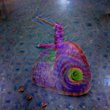
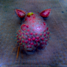
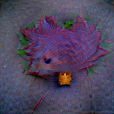
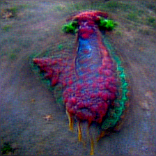
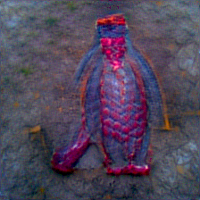
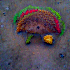
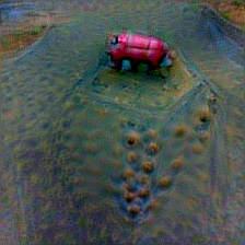
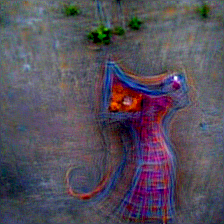
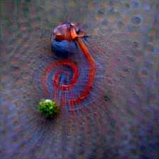
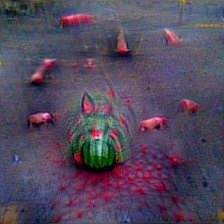
CLIPig animal transfer

Once the astonishment and the feeling of complete personal incompetence has diminished after reading the amazing article about DALL-E, i gathered some courage back and investigated the methods that OpenAI used to create those images.

DALL-E is based on the GPT3 transformer. The paper is overwhelmingly complex, not only in terms of the algorithms but also with regard to reducing and distributing computation across hundreds of expensive GPUs to allow training convergence within only weeks instead of years.

The major components of GPT3 and DALL-E are not publicly released so there’s no way for an average middle-class individual to reproduce those results. The CLIP network on the other hand, which was used to pick the best images produced by DALL-E, is available to the middle class.

So i started playing with it a couple of weeks ago which resulted in the CLIP Image Generator, a little framework for creating images out of the blue, using CLIP as an art critique.

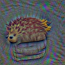
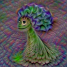
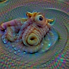
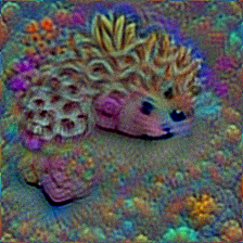
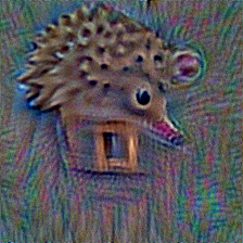
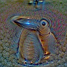
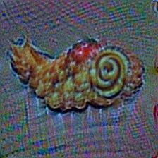
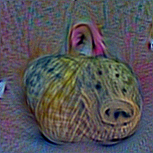
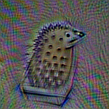
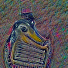
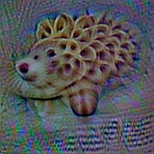
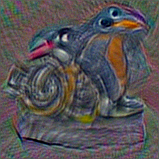
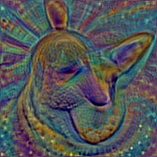
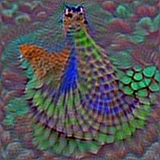
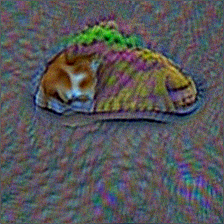
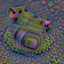
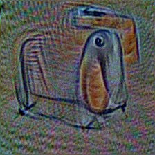
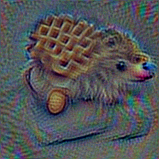
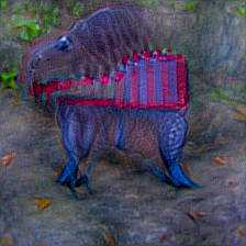
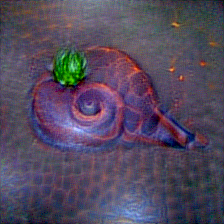
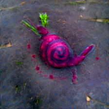
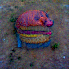
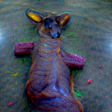
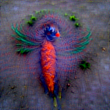
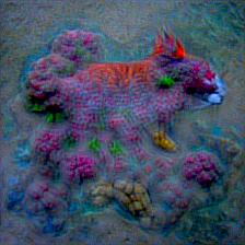
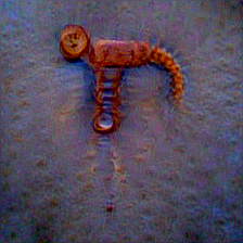
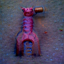
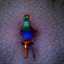
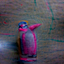
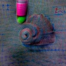
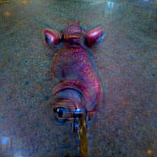
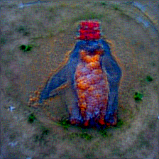
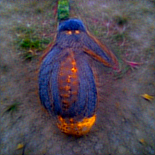
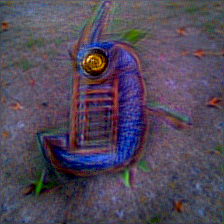
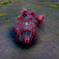
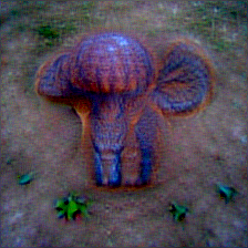
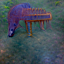
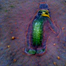
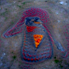
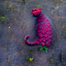
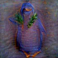
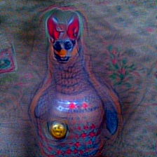
Below is a reproduction of the animal concept transfer experiment in the DALL-E article using only the CLIP network.

You can use the up and down cursor keys to select a thing and the 1 and 2 key respectively to select the rendering method.

Details

I chose the example because i liked the penguins made of piano so much. Some of them are really artistic in the sense that: If a human artist selects one of the top-ranked images it becomes true art.

When one interacts with the prompt selector in the article, the list of keywords and corresponding text prompts is printed to the web-console so it’s easy to reuse.

DALL-E vs. CLIPig

DALL-E creates images by completing a sentence, similar to GPT3, where each token describes an 8² pixel window. A sentence in natural language and optionally some initial image tokens are provided and DALL-E generates the next image tokens by the best of it’s knowledge.

In CLIPig, an image (starting with noise) is constantly updated to increase the similarity between it’s feature and a target feature, usually created via a natural language text prompt. The features are calculated by CLIP and the optimization of the feature loss, coupled with a few hand-designed transformations during each training step, may eventually lead to an image that a human does indeed recognize as the depiction of what the text prompt suggests.

Computation time and number of images

Each image shows CLIPig’s first try. There is no ranking among 512 different runs as in the DALL-E article because i simply can not afford the computation time. Rendering a single image took 137 seconds for method 1 and 194 seconds for method 2. There are 9 animals and 90 different things which resulted in a rendering time of 31 and 44 hours respectively. Multiplying that with 512 leads to several years of computation time. At 50 Watts/h. Which i don’t think reasonable at any rate.

I guess that generating an image with DALL-E only takes a few seconds as it is a completely different method.

Some experiments with ranking multiple runs where carried out. They are shown below. But first the two methods will be briefly described.

Method 1

A 224² pixel image is initialized with a bilinear-scaled 10² pixel noise. Some random rotation and a little noise is applied before each CLIP evaluation. During the first 10% of training, the resulting image is blurred after each training step. Below is the complete CLIPig configuration script.

epochs: 200
optimizer: rmsprob
learnrate: 1.0

init:
  mean: 0.33
  std: 0.03
  resolution: 10

targets:
  - batch_size: 10
    features:
      - text: a cat made of salami. a cat with the texture of a salami.
    transforms:
      - pad:
          size: 32
          mode: edge
      - random_rotate:
          degree: -30 30
          center: 0 1
      - mul: 1/2
      - mean: .5
      - noise: 1/10

postproc:
- blur:
    kernel_size: 3
  end: 10%

Method 2

The major difference to method 1 is the resolution. In the beginning of the training, a 8² pixel image is optimized. The resolution increases to 16², 32², 64², 128² and finally 224² pixels during the first half of the training. The idea behind this is that optimizing a very low resolution image will encourage CLIP to create proper objects in the first place without increasing the feature similarity through fine (adversarial) details. Once a nice object is rendered CLIP may work out the details.

As can be seen by comparing the images of the two methods, this resolution trick leads to a very different style.

The text prompt was shortened to the first sentence, ‘an animal made of thing.’ and the second sentence ‘an animal with the texture of a thing.’ was dropped because i subjectively liked most of the resulting images better.

Here’s the configuration:

epochs: 300
resolution: 
  - '{0: 8, 1: 8, 2: 16, 3: 32, 4: 64, 5: 128}.get(int(t*16), 224)' 
optimizer: rmsprob
learnrate: 1.0

init:
  mean: 0.3
  std: .01

targets:
  - batch_size: 10
    features:
      - text: a cat made of salami.
    transforms:
      - resize: 224
      - pad:
          size: 32
          mode: edge
      - random_rotate:
          degree: -20 20
          center: 0 1
      - random_crop: 224
      - mul: 1/3
      - mean: 0.5
      - bwnoise: 1/5*ti
    constraints:
      - blur: 
          kernel_size: 11
          start: 50%
      - saturation:
          below: 0.005

Ranking experiment

Images in CLIPig emerge by progressively massaging pixel planes into something that CLIP would rate as a high match to the target feature. The whole process is stochastic and each run produces a different image with a slightly different feature similarity.

In the following experiment two of the example text prompts have been rendered 512 times each. The image training was reduced to 20 epochs, instead of 200 or 300. The best 6 matches, according to CLIP, where selected and rendered for another 300 epochs.

Method 1 starts with 10x10 random pixels, so it’s already pointing CLIP to a certain space within the similarity should be increased.

Method 2 starts by generating a small (8x8, then 16x16) image to help CLIP concentrate on the proper position of objects before working on the details. In this case, the best 16x16 images where selected for further rendering. I did not see a lot of difference between many of those small images and stopped the initial runs at some point.

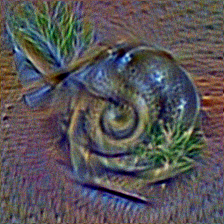
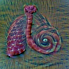
The following table shows each prompt’s (or method’s) 6 best images and 2 worst, rated after the initial run. The sim numbers show the rating results after the initial run on the left and after the final run on the right.

snail of harp (method 1)	penguin of piano (method 1)	penguin of piano (method 2)
best of 512 (csv)	best of 512 (csv)	best of 149 (csv)
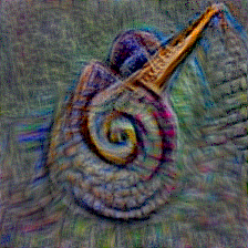#487 sim: 36.81 ⭢ 45.49	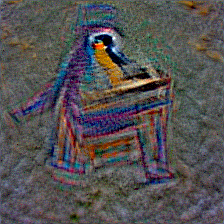#344 sim: 35.30 ⭢ 48.65	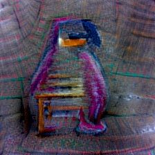#108 sim: 21.86 ⭢ 46.65
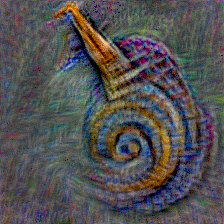#134 sim: 36.77 ⭢ 45.77	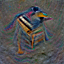#43 sim: 35.23 ⭢ 47.54	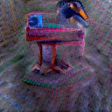#80 sim: 21.56 ⭢ 47.80
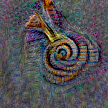#326 sim: 36.60 ⭢ 45.48	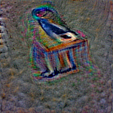#260 sim: 34.38 ⭢ 48.01	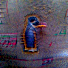#137 sim: 21.39 ⭢ 49.67
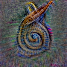#268 sim: 36.50 ⭢ 45.07	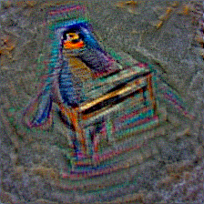#40 sim: 34.11 ⭢ 49.50	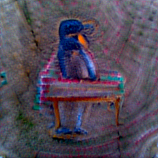#42 sim: 21.29 ⭢ 50.49
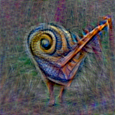#471 sim: 36.45 ⭢ 45.77	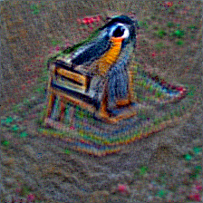#221 sim: 33.00 ⭢ 49.65	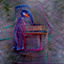#21 sim: 21.28 ⭢ 49.92
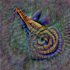#38 sim: 36.35 ⭢ 45.61	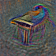#244 sim: 31.69 ⭢ 38.75	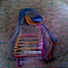#24 sim: 21.24 ⭢ 47.43
worst of 512	worst of 512	worst of 149
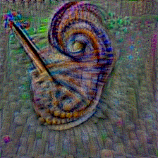#214 sim: 28.86 ⭢ 45.38	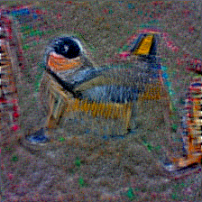#57 sim: 20.22 ⭢ 46.67	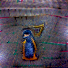#6 sim: 17.80 ⭢ 48.58
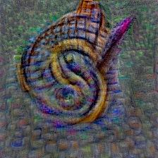#171 sim: 29.40 ⭢ 46.18	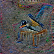#390 sim: 20.82 ⭢ 47.87	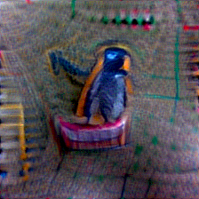#106 sim: 18.48 ⭢ 48.61

For comparison, the ratings of the respective DALL-E images are displayed below.

snail of harp (DALL-E)	penguin of piano (DALL-E)
best of 30 (csv)	best of 30 (csv)
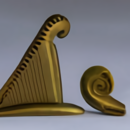#55 sim: 37.97	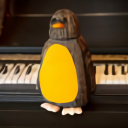#13 sim: 37.86
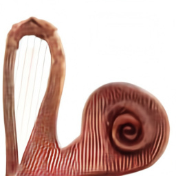#58 sim: 37.43	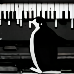#1 sim: 36.30
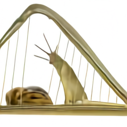#45 sim: 36.24	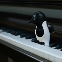#25 sim: 36.28
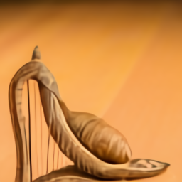#36 sim: 35.31	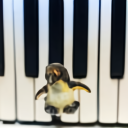#3 sim: 35.96
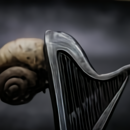#31 sim: 35.20	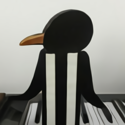#12 sim: 35.92
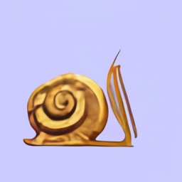#47 sim: 35.16	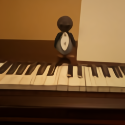#24 sim: 35.78
worst of 30
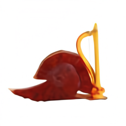#53 sim: 25.50	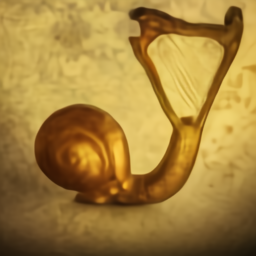#30 sim: 21.12
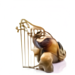#48 sim: 26.05	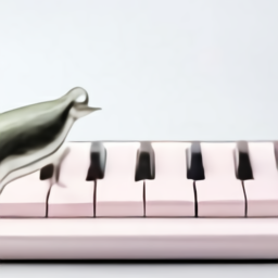#8 sim: 26.68

Conclusion

The CLIPig images are not nearly as good as the DALL-E samples, both in terms of quality and diversity of the composition idea.

The ranking experiment shows that it’s quite hard to create convincing shapes and forms just from noisy training on pixel planes.

Looking at the deviation of the initial and final ranking values, we can see that a couple of hundred epochs of training in CLIPig will raise the similarity value to high levels in almost any case, no matter the initial state of the image. The one exception being penguin #244 where the penguin is actually nicely coalescing with the piano but the fine boundaries and details could not be worked out.

The worst snails #214 and #171 have actually turned out quite interesting in the final training. The method 2 penguins #6 and #106 seem to raise the final similarity just by piano-ish background patterns.

Honestly, the amount of compute currently required for creating interesting images with a high probability is not worth the resources. So, without years of computation, here’s my: