<< nn-experiments
- Solving the "Very Selective Copying" problem with a Very Small Language Model
- Preliminary tests
- Number of operations versus number of layers
- Quick comparison with Mamba and LSTM
- Attention, please!
- Compare attention activation function
- Compare position of self-attention in 3-layers network
- Compare position of self-attention in 5-layers network
- 6-layers
Solving the "Very Selective Copying" problem with a Very Small Language Model ←
This is a very numeric continuation of a previous experiment. To get a grip on the details, please check "Selective Copying" first.
Basically, it's a synthetic question-answer dataset that requires some "computational" skill. See, if you can find out the rule by yourself:
NA: 2>1: AN
DQ: -1: Q
EJWHB: 3>5: EJBHW
ULHP: 3>4, 2>1: LUPH
YNP: 3>1, -3, 2>1: NP
EJACQ: 1>2, -1, +3: EAJCQ
YESBR: 3>5, 5>1, 1>5, 3>4: YEBRS
UXMP: -2, -3, 1>2, +2: MPU
Spoiler: First few letters are the program input, the numbers and operators are the program and answer, after the second colon, is the result of the program.
x>ymeans: exchangexth item withyth item.-xmeans: removexth item from memory and put it onto the stack.+xmeans: pop last item from stack and insert at positionx
I argue, that this dataset
- requires a large enough receptive field
- requires some cognitional ability to build up a history and to use it subsequently.
- should actually be called Selective Swapping
Preliminary tests ←
Just to get a feeling for the dataset, i took the best model from the "Selective Copying" experiment with a few parameter variations and ran it on questions that have an input length of 2 to 5 items and 1 to 5 operations:
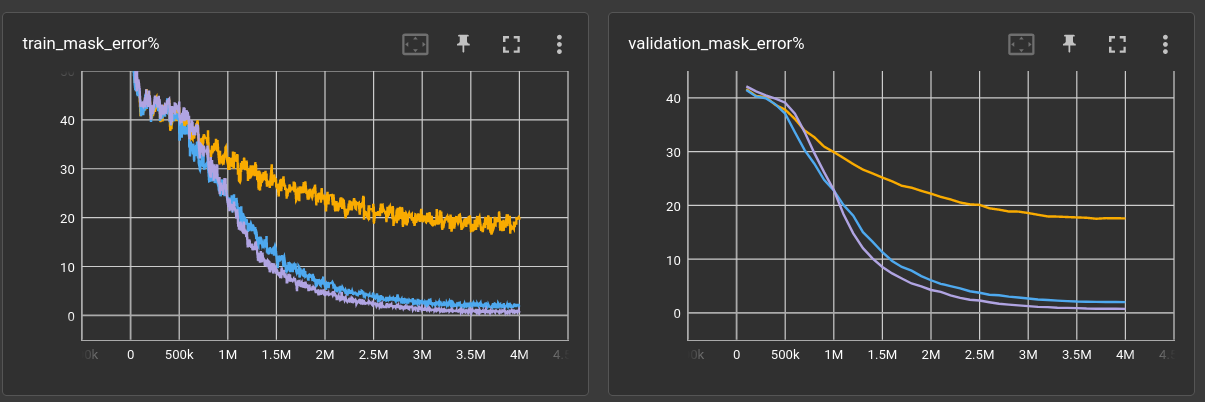
Training now takes 4 million steps, and could even be a bit longer. But generally, the loss curves seem to converge at about there.
| nitem | len | nops | l | ch | ks | dil | validation loss | validation_mask_error% | model params | train time (minutes) | throughput |
|---|---|---|---|---|---|---|---|---|---|---|---|
| 26 | 2,5 | 1,5 | 6 | 64 | 9 | 1,2,3,4,5,1 | 0.0525558 | 17.5876 | 237,952 | 15.30 | 4,358/s |
| 26 | 2,5 | 1,5 | 6 | 128 | 9 | 1,2,3,4,5,1 | 0.0365154 | 11.8352 | 918,272 | 10.76 | 6,195/s |
| 26 | 2,5 | 1,5 | 12 | 64 | 9 | 1,1,2,2,3,3,4,4,5,5,1,1 | 0.0076271 | 2.0063 | 459,520 | 27.05 | 2,464/s |
| 26 | 2,5 | 1,5 | 18 | 64 | 9 | 1,1,1,2,2,2,3,3,3,4,4,4,5,5,5,1,1,1 | 0.0028902 | 0.7583 | 681,088 | 39.80 | 1,675/s |
| 26 | 2,5 | 1,5 | 12 | 128 | 9 | 1,1,2,2,3,3,4,4,5,5,1,1 | 0.0028549 | 0.7205 | 1,803,776 | 18.81 | 3,543/s |
I'm using dilation all the time, because 1.) it's required for the receptive field of the 6-layer network and 2.) because it runs faster. For the 12 and 18-layer networks i just expanded the dilation settings without much thinking about it. (Actually i did think quite a bit about it but decided to evaluate good 12 or 18-layer dilation settings another time)
Here are examples from the validation set from the worst and the best performing network:
6-layer/32-chan: validation mask error 17.6% ←
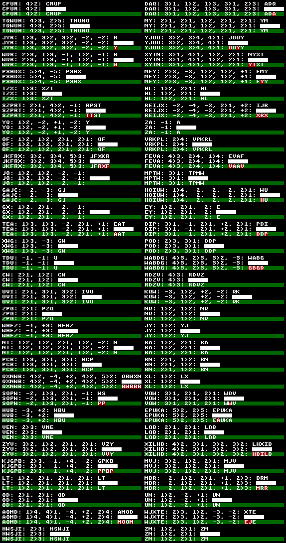
It is noticeable that long programs seem to be the problem for this network.
12-layer/128-chan: validation mask error 0.7% ←
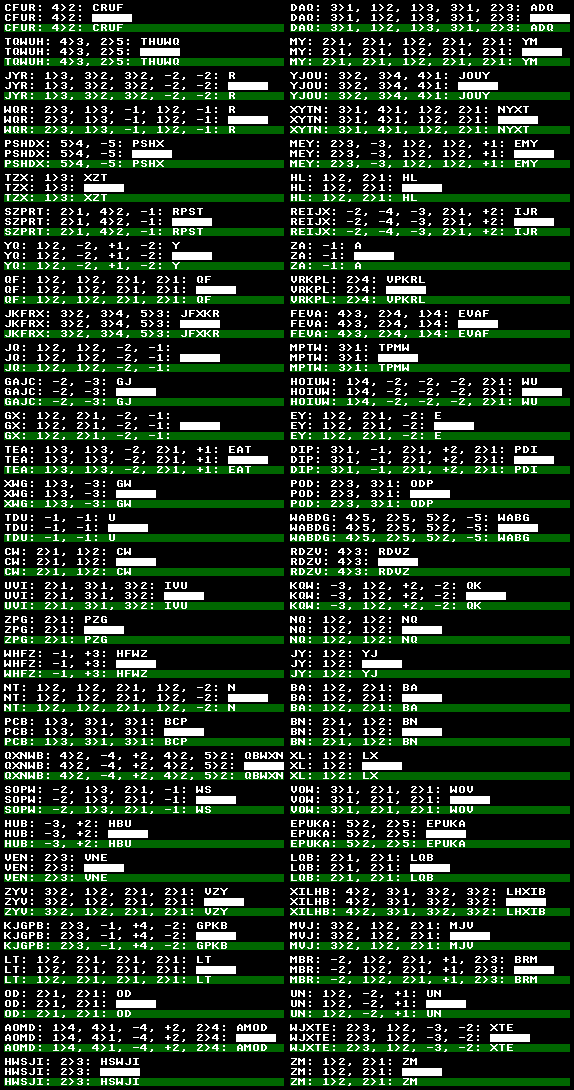
Wow! Everything correct, even the long ones!
Number of operations versus number of layers ←
The above example is a bit messy because it has a variable number of operations and
we don't know how many answers are fully correct, only how many characters.
So first, we add a new evaluation metric validation_sample_error%. While the mask error gives
the percentage of wrong characters within the mask area, the sample error gives the percentage
of wrong answers, even if only one character is wrong.
Further, to better evaluate the relationship between number of operations (length of the "program") and the number of layers in the network, i set a fixed number of operations.
I also dropped the stack operations (+/-) for now and made it all a bit tighter because
i'm not interested in the influence of the receptive field in this experiment.
Example data with 5 operations looks like this:
NPFKT:5>4 3>1 1>4 4>2 1>3:NFTPK
UKLRM:5>1 4>2 1>4 2>4 3>2:KLMRU
LCEWI:3>5 3>2 4>2 3>1 3>5:CWEIL
LRUPX:1>4 3>2 5>4 1>3 2>1:URPXL
UQJOR:5>4 2>5 5>4 4>3 2>5:URQJO
BYGMJ:5>4 4>3 2>3 5>2 5>3:BMJGY
PBNFM:3>5 5>1 1>3 2>3 5>3:MNPFB
TNEOL:1>3 4>1 4>1 4>3 5>3:ENLTO
ALEVT:1>2 2>1 2>1 4>2 4>3:LVAET
UIZNQ:3>4 2>3 5>3 4>1 1>5:INQUZ
Running the networks on 2, 3, 4 and 5 operations per question:
6-layer ←

12-layer ←

18-layer ←

And here is it all together in a table. The dilation settings are left out for readability.
They are 1,2,3,4,5,1 for the 6-layer, 1,2,3,4,5,1,2,3,4,5,1,1 for the 12-layer
and 1,2,3,4,5,1,2,3,4,5,1,2,3,4,5,1,1,1 for the 18-layer network.
| nitem | len | nops | l | ch | ks | validation loss | validation_mask_error% | validation_sample_error% | model params | train time (minutes) | throughput |
|---|---|---|---|---|---|---|---|---|---|---|---|
| 26 | 5 | 5 | 6 | 64 | 9 | 0.23663 | 71.9705 | 99.9104 | 237,952 | 58.04 | 1,145/s |
| 26 | 5 | 5 | 12 | 64 | 9 | 0.208893 | 63.6883 | 99.4327 | 459,520 | 40.0 | 1,660/s |
| 26 | 5 | 5 | 18 | 64 | 9 | 0.163338 | 50.2667 | 98.547 | 681,088 | 99.0 | 670/s |
| 26 | 5 | 4 | 6 | 64 | 9 | 0.185987 | 48.7739 | 98.5967 | 237,952 | 15.1 | 4,413/s |
| 26 | 5 | 4 | 12 | 64 | 9 | 0.0415355 | 8.8953 | 37.8682 | 459,520 | 26.03 | 2,561/s |
| 26 | 5 | 3 | 6 | 64 | 9 | 0.00458625 | 0.559315 | 2.75677 | 237,952 | 7.32 | 9,109/s |
| 26 | 5 | 4 | 18 | 64 | 9 | 0.000329348 | 0.0378185 | 0.189092 | 681,088 | 37.13 | 1,795/s |
| 26 | 5 | 3 | 18 | 64 | 9 | 1.86865e-06 | 0 | 0 | 681,088 | 5.07 | 13,139/s |
| 26 | 5 | 3 | 12 | 64 | 9 | 3.1804e-06 | 0 | 0 | 459,520 | 11.5 | 5,796/s |
| 26 | 5 | 2 | 18 | 64 | 9 | 4.39884e-07 | 0 | 0 | 681,088 | 15.3 | 4,357/s |
| 26 | 5 | 2 | 6 | 64 | 9 | 5.3105e-07 | 0 | 0 | 237,952 | 7.15 | 9,319/s |
| 26 | 5 | 2 | 12 | 64 | 9 | 1.0319e-06 | 0 | 0 | 459,520 | 11.3 | 5,900/s |
Something is obviously very strange. None of the networks can handle 5 operations. But some of them just did in the last experiment??
What i really like about this neural net research is that one often gets along with intuition only. We simply don't know enough until all tests are made, which probably never happens. However, in this case, i would argue that a 5 operations sequence is just too long for the network to learn the task in reasonable time. Put yourself into the eyes of the model. The training algorithm constantly tells you:
If you see this:
PHMTW:5>3 2>3 5>4 5>3 1>3:?????you should output that:PHMTW:5>3 2>3 5>4 5>3 1>3:TWPMH
on and on ... for millions of examples. Now, for a human, maybe a programmer even, this should be solvable pretty quick. Once you have seen 10 examples, you can be sure what the algorithm is. But for a neural network trained with stochastic gradient descend it is basically a brute-force approach. It's like: Hey network, you gotta lot of parameters, that's fine, now if you see this X, and you should output that Y, there is a chance that inreasing this one parameter while decreasing that other one would help you to output the correct answer, the next time you see the same question. And on and on...
Once again, reasoning from intuition, the network can probably learn the task much easier when it has some easier examples in the dataset. Schools and such also don't teach children algebra by starting with: What is the answer to 7 + 4 + 9 + 2 + 6 = ??
Following, the training set contains questions with 2 to 5 operations, e.g.:
HGOKX:3>1 5>4:OGHXK
CXZMN:5>4 2>5:CMZNX
RMYTC:2>1 4>5 4>2:MCYRT
DNAHL:1>3 3>4 1>2 4>1 3>2:DHANL
HSBQA:4>5 4>5:HSBQA
DTFKS:4>5 3>2 4>5 5>1:SFTKD
UXGJN:4>2 1>2 1>4 3>1 3>2:GXUJN
and the validation set still holds the same 5-operations-only questions for which all networks have failed previously.
Here's the loss and error curves of the 18-layer network trained with 5 and 2-5 operations:
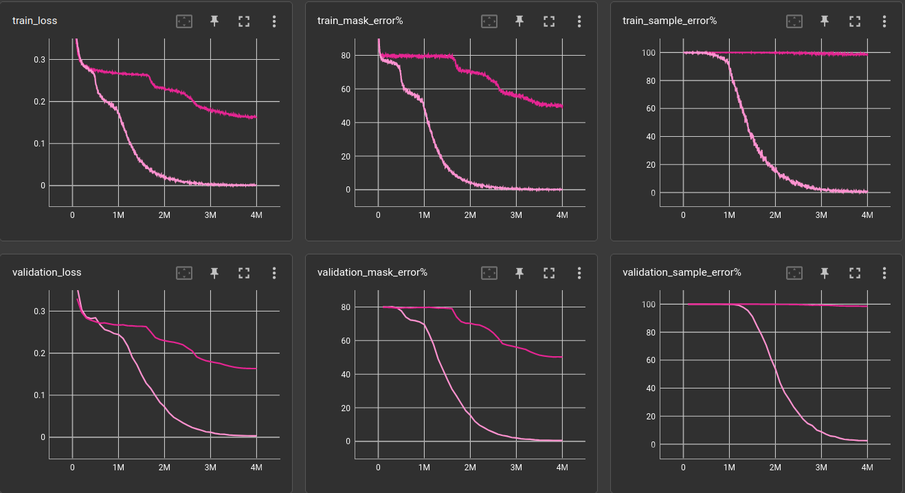
The bright one is the brighter one. Indeed, the 18-layer gets down to 2.5% sample error. It is able to solve the task (to a degree), it could just not learn it from the previous dataset. One could argue, though, that it would eventually learn the task just from the 5-operations examples but it would probably take 10 to 100 times more computation / CO2-emissions / floodings / draughts / you-name-it.
| nitem | len | nops | val-nops | l | ch | ks | validation loss | validation_mask_error% | validation_sample_error% | model params | train time (minutes) | throughput |
|---|---|---|---|---|---|---|---|---|---|---|---|---|
| 26 | 5 | 2,5 | 5 | 6 | 64 | 9 | 0.208661 | 60.0816 | 99.5123 | 237,952 | 16.55 | 4,027/s |
| 26 | 5 | 2,5 | 5 | 12 | 64 | 9 | 0.0322987 | 6.74761 | 27.3885 | 459,520 | 27.59 | 2,416/s |
| 26 | 5 | 2,5 | 5 | 18 | 64 | 9 | 0.00329394 | 0.565287 | 2.5577 | 681,088 | 41.25 | 1,615/s |
We can see from the table, that the 12 and especially the 6-layer networks are struggling. Looking at the plots of the 6-layer networks trained with 5 and 2-5 operations, we can see that the mask error decreases by a good amount but actual sample error stays roughly the same. It learned to put some letters at the right place but still fails for almost every validation sample:
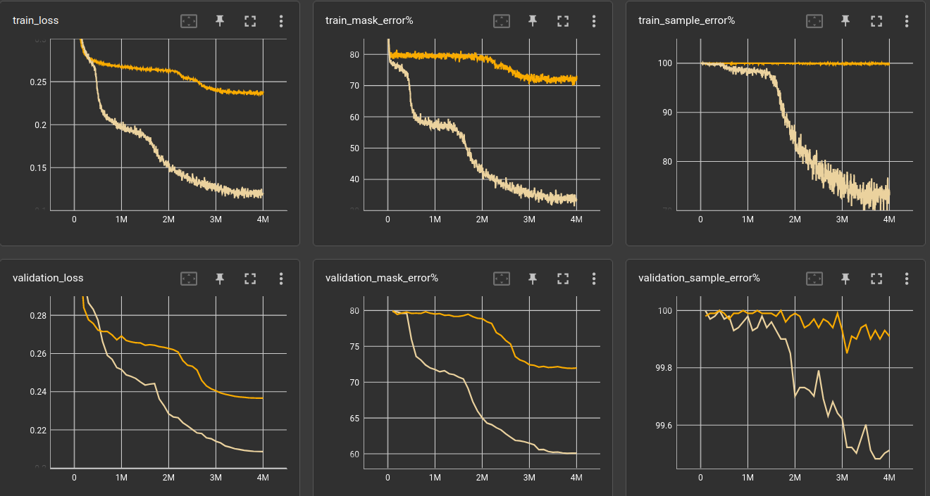
- Quick takeaway: Put also some easy examples in the training set!
The curves suggest, however, that training has not yet converged. There are sure a few more per-mille to squeeze out.
This is a good point of origin for further experimentation. Can we get the 6-layer network to solve the 5-operations Very Selective Copying problem,
- without adding so many modules that it actually resembles a 12-layer network
- without making it slower to execute than the 12-layer network
- bonus: by keeping the number of model parameters equal or even lower
In other words, is there a trick, maybe to pass data around in a different way, that strongly increases the computational performance?
Quick comparison with Mamba and LSTM ←
Just for another set of baselines, i tried the state-spaces/Mamba (yet the slow version because the fast doesn't run on my system) and the all-beloved LSTM (the pytorch implementation).
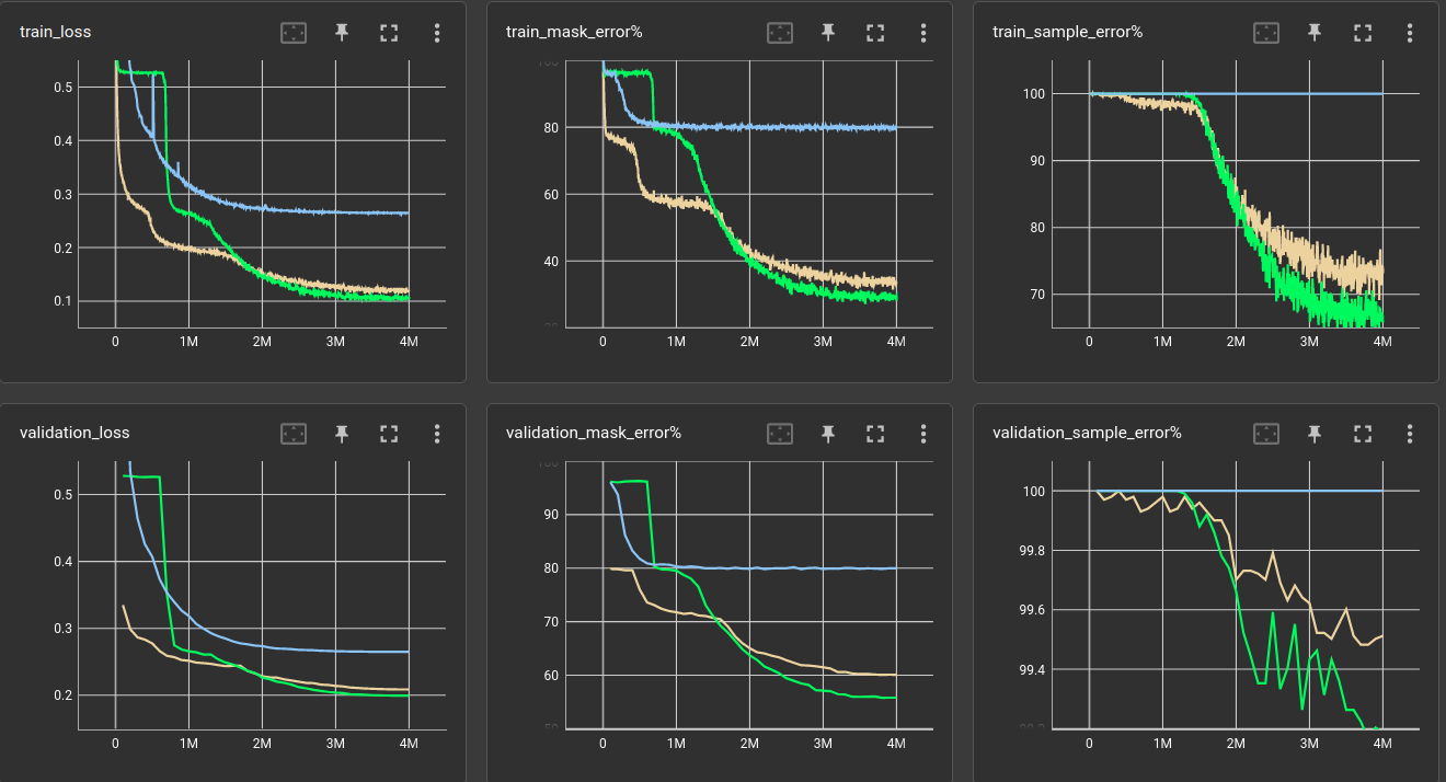
The yellow/brownish is the 6-layers model from above, green is Mamba and blue the LSTM. All of them have 6 layers
| nitem | len | nops | val-nops | l | model | validation loss | validation_mask_error% | validation_sample_error% | model params | train time (minutes) | throughput |
|---|---|---|---|---|---|---|---|---|---|---|---|
| 26 | 5 | 2,5 | 5 | 6 | LSTM hidden_size=64 | 0.264829 | 79.9602 | 100 | 216,064 | 6.72 | 9,926/s |
| 26 | 5 | 2,5 | 5 | 6 | Conv1d channels=64 (from above) | 0.208661 | 60.0816 | 99.5123 | 237,952 | 16.55 | 4,027/s |
| 26 | 5 | 2,5 | 5 | 6 | MAMBA d_model=32 d_state=16 | 0.199433 | 55.8081 | 99.1839 | 67,936 | 126.56 | 526/s |
- None of these especially-crafted models reached a significant performance gain.
- To be fair: The Mamba model is very small compared to the Conv1d, just 28% of parameters. Though it manages to consume 7.8x more computation time. The first tiny drop in sample error occurred after 1 hour of training and i do not have the patience today to train an equally-sized Mamba for comparison. (The dynamics of the curves suggest, that it would not change much)
- The LSTM basically archived nothing (though equal-sized). It's about as bad as the 6-layer Conv1d with only 5-operations questions in the training set. At least, it's blazinlgy fast!
- Disclaimer: I do not know any good practices about using or training LSTMs or Mambas and surely made some grave mistake..
Back to the residual CNN. To find some interesting method, quick, i switched to 3 operations and 3-layer networks. The above condition holds as well. The 3-layer network is not able to solve the 3-operations task in the validation set, but it only takes about 2 minutes to find out:
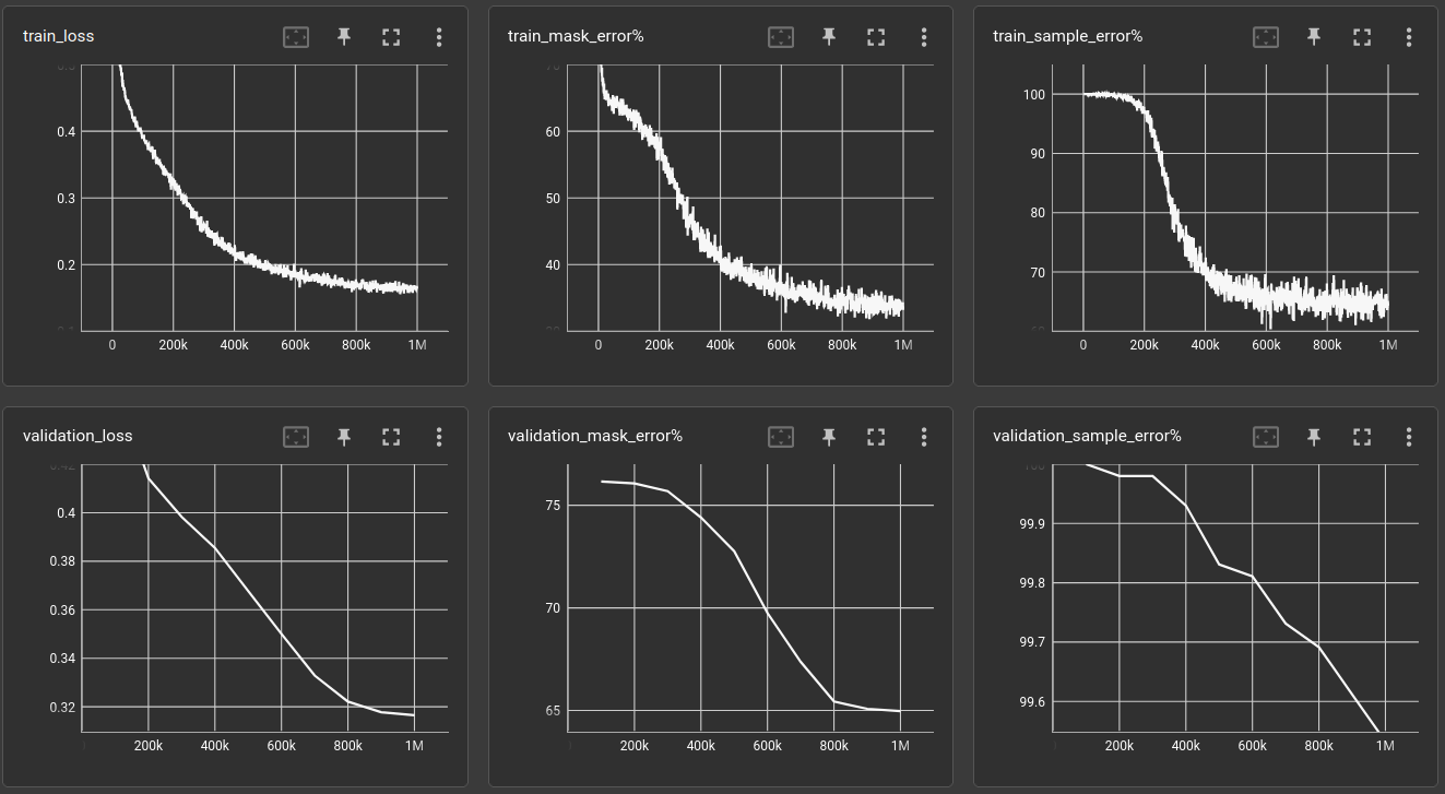
The validation sample error stays roughly at 100%.
I tried a couple of things, like adding cross-residual connections, e.g. from layer 1 to layer 3, which did not noticeably improve performance. Also tried learnable weights, so that each layer can use as input a weighted mix of all previous layers. Was not much help either, also not for the 6-layer networks.
Attention, please! ←
UPDATE: After revision of the used experiment files, i just painfully realized that some of the below findings are wrong. In short, i forgot to put the QKV and the attention activation variables to the network constructor and as such, the tables comparing these values show something completely different. There is obviously so much deviation between similar runs, that the results fooled me to make conclusions about best parameters, although there was nothing to compare...
I'm leaving the manuscript below as it is, as a reminder how stupid the search for explanations was, without a scientific basis. However, the corrections are linked at the appropriate places.
Eventually i remembered that, in an age-old lecture by Geoff Hinton, he argued that for this particular case he showed, the network can not succeed without a cell-wise multiplication somewhere. Then there is this relatively recent Schlag, Irie & Schmidhuber paper (2102.11174) "Linear Transformers Are Secretly Fast Weight Programmers", which states: Fast Weight Programmers (FWPs, 1991) program their fast weight memories through sequences of outer products between self-invented key and value patterns. I just like the self-invented notion.
To make it short, i plugged a torch.nn.MultiheadAttention module into the last layer, such that
the 1d-convolution, which normally outputs 64 channels, now outputs 128 channels, which are split
into 64 query and 64 key channels and the attention-values are the input of the layer.
The pseudo-code looks like:
qk = Conv1d(64, 128)(inp)
q, k = split(qk, 64)
outp = attention(q=q, k=k, v=inp)
Not shown is, that q, k and v (which are each of shape [B, C, L]) are transposed before the
attention to move the channels (C) to the last dimension ([B, L, C]), and make it a
channel-wise attention.
The pytorch MultiheadAttention has a predefined fixed length, because it adds bias and
a couple of other learnable parameters, so it has to be used channel-wise, since we don't
want to fix the sequence length that the network processes.
But wait, the Fast Weight Programmers-paper, said self-invented keys and values not self-invented keys and queries. So, for completeness, let's test all the combinations
self-invented keys and values ←
kv = Conv1d(64, 128)(inp)
k, v = split(kv, 64)
outp = attention(q=inp, k=k, v=v)
self-invented queries and values ←
qv = Conv1d(64, 128)(inp)
q, v = split(qv, 64)
outp = attention(q=q, k=inp, v=v)
self-invented queries, keys and values ←
qkv = Conv1d(64, 192)(inp)
q, k, v = split(qkv, 64)
outp = attention(q=q, k=k, v=v)
Unfortunately, the validation sample error varies quite a lot for each run of the same network:
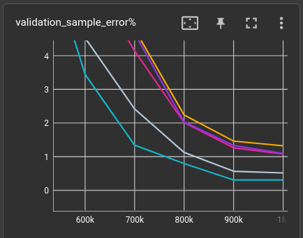
So i'm doing 5 runs each and report the average. That's 80 runs for this messy plot and the table below!
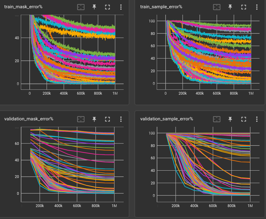
Each run has the same validation set but different training sets and initial network weights. (reproduce with convtext-qa-program-3ops-attn-invent.yml @ 613064ad)
UPDATE: Please check the correction!
| qkv | attn | validation loss | validation_mask_error% | validation_sample_error% | validation_sample_error% (std) | model params | train time (minutes) | throughput |
|---|---|---|---|---|---|---|---|---|
| 0,0,0 | 0.316488 | 64.9682 | 99.5322 | 176,320 | 2.24 | 7,434/s | ||
| QK | 0,0,1 | 0.323012 | 63.3965 | 99.4765 | 0.8504 | 246,272 | 1.77 | 9,437/s |
| QKV | 0,0,1 | 0.287839 | 56.5426 | 93.1568 | 14.4636 | 246,272 | 1.86 | 8,950/s |
| KV | 0,0,1 | 0.219660 | 41.3674 | 86.0450 | 16.6931 | 246,272 | 1.88 | 8,884/s |
| QV | 0,0,1 | 0.197362 | 38.2166 | 75.5036 | 29.8328 | 246,272 | 2.1 | 7,963/s |
| QV | 0,0,4 | 0.151719 | 29.0418 | 61.0768 | 47.2315 | 246,272 | 1.93 | 8,661/s |
| QK | 0,0,4 | 0.048829 | 8.2794 | 32.6791 | 32.2507 | 246,272 | 1.93 | 8,653/s |
| QKV | 0,0,4 | 0.051348 | 8.4331 | 31.2838 | 42.0001 | 246,272 | 1.88 | 8,863/s |
| KV | 0,0,4 | 0.048607 | 8.0497 | 30.4976 | 36.3580 | 246,272 | 1.87 | 8,905/s |
| QK | 0,0,8 | 0.050850 | 8.9243 | 25.5235 | 40.7858 | 246,272 | 1.9 | 8,771/s |
| QV | 0,0,8 | 0.034589 | 6.0991 | 18.8754 | 38.8027 | 246,272 | 1.96 | 8,490/s |
| QKV | 0,0,8 | 0.024016 | 3.6755 | 15.4618 | 27.0721 | 246,272 | 1.92 | 8,698/s |
| KV | 0,0,8 | 0.002678 | 0.2691 | 1.3395 | 1.0593 | 246,272 | 2.03 | 8,228/s |
| QV | 0,0,True | 0.002325 | 0.2683 | 1.2997 | 0.5423 | 229,632 | 1.77 | 9,449/s |
| KV | 0,0,True | 0.002089 | 0.2316 | 1.1504 | 0.4276 | 229,632 | 1.67 | 9,973/s |
| QKV | 0,0,True | 0.001974 | 0.2157 | 1.0648 | 0.3161 | 229,632 | 1.84 | 9,104/s |
| QK | 0,0,True | 0.001686 | 0.1755 | 0.8638 | 0.4294 | 229,632 | 1.62 | 10,301/s |
-
qkvis one of the self-invented methods above. e.g.QKmeans,Query andKey come from convolution,Value is unprocessed. -
attn: 0,0,0is no attention -
attn: 0,0,Xis multi-head attention in final layer withXheads -
attn: 0,0,Trueis a self-built attention, loosely following equation 6 in Transformers are RNNs: Fast Autoregressive Transformers with Linear Attention (2006.16236]). In contrast to the torchMultiheadAttention, The self-made function does not have any parameters and works on sequences and channels of any length.def attn(q: torch.Tensor, k: torch.Tensor, v: torch.Tensor) -> torch.Tensor: q = F.elu(q) + 1. k = F.elu(k) + 1. return q @ (k.permute(0, 2, 1) @ v) / (v.shape[-1] * v.shape[-2]) -
(std)is the standard variation given for the validation sample error
So,
- the average validation sample error is smallest for the self-built, self-invented QK attention, followed by all the other self-built variants.
-
Best number-of-heads for pytorch attention seems to be 8,
- and the only performing self-invented combination seems to be Key/Value, as stated in the FWP paper..
- The absolutely-prooven-to-not-working model is pytorch attention with QK and heads=1.
- Generally, the pytorch attention module is very unstable in this experiment. Look at the error deviations! Occasionally, one of 5 runs produced a far better validation sample error than 0.8%.
Admittedly, there is something about this so-called Attention that works pretty well. Thinking in terms of the receptive field, these two dot-products in the attention formula bring every point in the sequence in contact with every other point, in a way that makes some sense. How exactly it makes sense, i can not tell. That's why i run these tests.
Compare attention activation function ←
The above activation function in the self-built attention module, elu(x) + 1, is suggested
by the authors (2006.16236), mainly because it needs
to be >= 0 and the elu gives a smooth gradient (unlike relu).
The Fast Weight Programmers-paper (2102.11174) suggests to replace this function with a more sparsity & orthogonality - aimed Deterministic Parameter-Free Projection (DPFP). Comparing the two activations for the 3-operators, 3-layers, 1-million-steps setup, averaged over 5 runs each, gives:
UPDATE: Check the correction!
| qkv | attn | attnact | validation loss | validation_mask_error% | validation_sample_error% | validation_sample_error% (std) | model params | train time (minutes) | throughput |
|---|---|---|---|---|---|---|---|---|---|
| QK | 0,0,True | dpfp | 0.00149588 | 0.164013 | 0.79816 | 0.538314 | 229,632 | 1.56 | 10,723/s |
| QK | 0,0,True | elu+1 | 0.00110781 | 0.091162 | 0.44785 | 0.211001 | 229,632 | 1.52 | 10,981/s |
Well, there is certainly a more powerful activation to be found for this particular task..
Compare position of self-attention in 3-layers network ←
Placing the best (most consistent) attention method from above into all the layers:
| qkv | attn | validation loss | validation_mask_error% | validation_sample_error% | validation_sample_error% (std) | model params | train time (minutes) | throughput |
|---|---|---|---|---|---|---|---|---|
| QK | T,0,0 | 0.292424 | 54.8229 | 99.1043 | 0.0962 | 229,632 | 2.88 | 5,788/s |
| QK | T,T,0 | 0.196146 | 39.6819 | 95.0159 | 0.6247 | 282,944 | 2.93 | 5,681/s |
| QK | T,T,T | 0.088230 | 17.0322 | 57.3487 | 29.2807 | 336,256 | 2.02 | 8,247/s |
| QK | 0,T,0 | 0.053625 | 8.9275 | 38.6146 | 8.3909 | 229,632 | 2.77 | 6,011/s |
| QK | 0,0,T | 0.001912 | 0.2161 | 1.0648 | 0.5693 | 229,632 | 1.54 | 10,827/s |
| QK | 0,T,T | 0.001125 | 0.1361 | 0.6926 | 1.2740 | 282,944 | 1.80 | 9,275/s |
| QK | T,0,T | 0.000185 | 0.0079 | 0.0437 | 0.0341 | 282,944 | 1.71 | 9,744/s |
Well, how can we explain that? It's very unfortunate that there is no obvious rule popping out, where to put the attention layers, except that there should be one in the final layer.
Or do you instantly know how to setup a 5-layer network for the 5-operations task, now?
Compare position of self-attention in 5-layers network ←
For efficiency, keep the above dataset (and the 1 million steps of training),
and use a 5-layer network with dilation=[2, 3, 4, 5, 1] to try all the attention-permutations.
| qkv | attn | validation loss | validation_mask_error% | validation_sample_error% | model params | train time (minutes) | throughput |
|---|---|---|---|---|---|---|---|
| QK | 0,0,0,0,0 | 0.226301 | 50.4797 | 98.7162 | 282,944 | 2.92 | 5,705/s |
| QK | T,T,T,T,T | 0.168785 | 32.6393 | 91.9686 | 549,504 | 2.88 | 5,783/s |
| QK | T,0,0,0,0 | 0.160457 | 29.9224 | 87.0521 | 336,256 | 3.16 | 5,276/s |
| QK | T,T,T,T,0 | 0.143025 | 25.5971 | 83.1111 | 496,192 | 3.67 | 4,545/s |
| QK | T,T,T,0,0 | 0.131017 | 23.9471 | 80.4638 | 442,880 | 3.47 | 4,804/s |
| QK | T,T,0,0,0 | 0.119354 | 22.0004 | 75.7564 | 389,568 | 3.3 | 5,053/s |
| QK | T,0,0,T,0 | 0.103017 | 18.4912 | 69.4068 | 389,568 | 3.38 | 4,927/s |
| QK | T,T,0,T,0 | 0.0981063 | 17.9598 | 66.9984 | 442,880 | 3.49 | 4,769/s |
| QK | T,0,T,0,0 | 0.0658464 | 11.9805 | 50.3881 | 389,568 | 3.36 | 4,956/s |
| QK | T,0,T,T,T | 0.0689705 | 12.0979 | 49.4128 | 496,192 | 2.63 | 6,327/s |
| QK | T,T,T,0,T | 0.0544455 | 9.24164 | 40.2170 | 496,192 | 2.63 | 6,334/s |
| QK | 0,T,0,0,0 | 0.0165344 | 2.36266 | 11.2162 | 336,256 | 3.17 | 5,251/s |
| QK | T,0,T,T,0 | 0.0127326 | 1.93471 | 9.40486 | 442,880 | 3.57 | 4,674/s |
| QK | 0,T,T,T,T | 0.00333168 | 0.427946 | 2.15963 | 496,192 | 2.56 | 6,512/s |
| QK | 0,T,0,T,0 | 0.00353792 | 0.376194 | 1.88097 | 389,568 | 3.36 | 4,957/s |
| QK | 0,T,T,0,0 | 0.00345656 | 0.350318 | 1.75159 | 389,568 | 3.42 | 4,866/s |
| QK | T,T,0,T,T | 0.00226949 | 0.248806 | 1.29379 | 496,192 | 2.59 | 6,447/s |
| QK | 0,0,T,0,0 | 0.00188953 | 0.181131 | 0.915605 | 336,256 | 3.24 | 5,138/s |
| QK | 0,T,T,T,0 | 0.00184384 | 0.173169 | 0.885748 | 442,880 | 3.53 | 4,723/s |
| QK | 0,0,T,T,0 | 0.00132653 | 0.095541 | 0.477707 | 389,568 | 3.23 | 5,153/s |
| QK | T,0,0,T,T | 0.000828459 | 0.083598 | 0.417994 | 442,880 | 2.43 | 6,846/s |
| QK | 0,T,0,T,T | 0.000377713 | 0.035828 | 0.189092 | 442,880 | 2.46 | 6,767/s |
| QK | 0,0,0,T,0 | 0.000290391 | 0.0199045 | 0.0995223 | 336,256 | 3.11 | 5,354/s |
| QK | 0,0,T,T,T | 0.000282769 | 0.0199045 | 0.0995223 | 442,880 | 2.51 | 6,644/s |
| QK | T,T,0,0,T | 0.000122952 | 0.0159236 | 0.0796178 | 442,880 | 2.41 | 6,913/s |
| QK | 0,0,T,0,T | 0.000144108 | 0.0119427 | 0.0696656 | 389,568 | 2.31 | 7,203/s |
| QK | T,0,T,0,T | 0.000167425 | 0.00796178 | 0.0398089 | 442,880 | 2.5 | 6,664/s |
| QK | 0,0,0,0,T | 6.164e-05 | 0.00398089 | 0.0199045 | 336,256 | 2.04 | 8,179/s |
| QK | 0,T,0,0,T | 6.42146e-05 | 0.00398089 | 0.0199045 | 389,568 | 2.26 | 7,376/s |
| QK | 0,T,T,0,T | 0.00010805 | 0.00398089 | 0.0199045 | 442,880 | 2.5 | 6,675/s |
| QK | T,0,0,0,T | 0.000154807 | 0.00398089 | 0.0199045 | 389,568 | 2.33 | 7,141/s |
| QK | 0,0,0,T,T | 2.67664e-05 | 0 | 0.00995223 | 389,568 | 2.24 | 7,453/s |
Okay okay, there is some slight pattern for arrangement of the self-attention modules emerging.
Now pick the best ones and train and test against 5-operations questions (at 4 million training steps):
| qkv | attn | validation loss | validation_mask_error% | validation_sample_error% | model params | train time (minutes) | throughput |
|---|---|---|---|---|---|---|---|
| QK | T,0,T,0,T | 0.107469 | 29.7174 | 87.2711 | 442,880 | 10.17 | 6,553/s |
| QK | 0,T,T,0,T | 0.0795734 | 21.7874 | 74.3432 | 442,880 | 10.03 | 6,648/s |
| QK | T,0,0,0,T | 0.0692764 | 18.6744 | 68.2524 | 389,568 | 9.57 | 6,965/s |
| QK | 0,T,0,0,T | 0.0635093 | 16.5983 | 61.6939 | 389,568 | 9.63 | 6,926/s |
| QK | 0,0,T,0,T | 0.0525193 | 14.9960 | 58.0812 | 389,568 | 9.37 | 7,117/s |
| QK | 0,0,0,0,T | 0.0072723 | 1.72572 | 8.1110 | 336,256 | 8.09 | 8,245/s |
It's still not completely sufficient. Let's switch back to 6-layer networks, again copying the best attention-settings, although, there is only one performing okay-ish, the others are worse than 50% error.
6-layers ←
| qkv | attn | validation loss | validation_mask_error% | validation_sample_error% | model params | train time (minutes) | throughput |
|---|---|---|---|---|---|---|---|
| QK | T,0,0,0,0,T | 0.0529652 | 14.0844 | 54.9562 | 442,880 | 10.39 | 6,419/s |
| QK | 0,T,0,0,0,T | 0.0196075 | 4.79498 | 21.666 | 442,880 | 14.6 | 4,566/s |
| QK | 0,0,0,T,0,T | 0.0143111 | 3.58081 | 16.5705 | 442,880 | 14.5 | 4,599/s |
| QK | 0,0,T,0,0,T | 0.0136107 | 3.27826 | 15.2767 | 442,880 | 14.49 | 4,601/s |
| QK | 0,0,0,0,T,T | 0.00143896 | 0.254777 | 1.27389 | 442,880 | 14.59 | 4,569/s |
| QK | 0,0,0,0,0,T | 6.6917e-05 | 0.00995223 | 0.0597134 | 389,568 | 13.82 | 4,823/s |
Well, i'm a bit tired of this topic right now.
Let's wrap the findings up, quickly:
- a 6-layer network can solve the 5-operations task, if we add self-attention to the last layer.
- The number of model parameters increased from 237,952 to 389,568 (because i still used the 13-kernels from the 3-layers experiments and the one 64-128 convolution for the self-invented QK)
- The training time increased from 14 to 17 minutes.
- Validation sample error decreased from 99% to 0.06%
- Is this a passable building block for a Very Small Language Model? I might have said yes but right now i say: Don't know, have to test it...
A little graphical disorder at the end of the day:
